Cross Sectional Astronomy

My research this summer came to an end last week with a seminar I presented at along with many other students in Caltech's Summer Undergraduate Research Program. In addition to presenting my work with Monte Carlo simulations, I also attended talks given by other students doing research in astronomy and physics.

Many of the astronomy projects I learned about focused on creating software for recognizing and analyzing different astronomical phenomena, from variable stars to pulsars and contact binary systems. Many large-scale sky surveys, such as the Palomar Transient Factory and the Sloan Digital Sky Survey, produce a wealth of data on astronomical objects. Computers are often the best way to analyze the abundance of data produced by these surveys in order to identify interesting targets for follow-up study. But why do astronomers need these huge sky surveys and millions of target objects to study?

Analyzing how any population changes over time, whether it is a population of people, stars, or starfish, is a common problem in many areas of science. It can be a tricky problem too, especially when trying to tease out correlation and causation from subtle differences between subgroups of the population. There are two main study methodologies for dealing with this problem: longitudinal studies and cross sectional studies.

Longitudinal studies are the intuitive approach to learning how a population changes over time: just watch as the population (or more realistically, a random sample of the population) evolves naturally. It makes sense, but it's difficult in a lot of situations. For example, longitudinal studies of humans take dedication and decades of research. For phenomena with long lifespans, such as stars, this type of study is simply impossible--the stars vastly outlast human lives and even human civilizations!

Cross sectional studies instead study many individuals in the population at the same time. Each individual represents an individual in a slightly different stage of evolution, with slightly different characteristics; a random sample provided by nature. In humans, an example of a cross sectional study is gathering pictures of many different individuals at different ages in order to examine how appearance changes with age.

Since astronomers only have access to a snapshot of the universe as it appears today, cross sectional studies are what astronomers use to study populations of stars. The most famous example of a cross sectional study is the Hertzsprung-Russel diagram, a plot that correlates star surface temperatures (or colors) with their luminosities. The diagram shows stars in different stages of their evolution, from main sequence stars to red giants and white dwarves, along with stars in transitional states between these major milestones.With the diagram, we can trace the development of different types of stars, and how this development changes with different intrinsic properties of the star (mass turns out to be the most important property in determining the ultimate fate of a star).

There are some problems with the cross sectional approach. For example, age itself may correlate with the evolution of the population in question. In the human example, improving health as time goes on might manifest itself in physical differences, such as an increase in height, between generations that are not caused by the aging process itself. In astronomy, a star that is now nearing the end of its life formed in a quite different universe than a protostar that has just reached the main sequence. We know from theoretical models that the concentration of metals in the universe has increased with time as stars convert hydrogen and helium into heavier elements. Luckily, we can attempt to correct for these effects. Due to the finite speed of light and the vast size of the universe, by looking further and further away, we effectively look back in time. This can help us to determine how conditions were different for older stars when they formed, when compared to stars which are forming today.

Having a large sample size is important in a cross sectional study because it ensures that a representative sample is available and than no important features of the population will be missed. Cross sectional methods and large samples provided by surveys help astronomers to discover how stars age, correlate properties among different populations of stars, and provide experimental confirmation of hypotheses for many types of astronomical objects. There is still much to be learned about a variety of astronomical systems--stars, planets, and more.

DIY Random Distributions

In this post, I explained how to generate a random, uniform distribution of points on a disk. That problem turns out to be a special case of a more general technique that can be used to generate random numbers with any probability distribution you want. As a bonus, it also explains the seemingly-magical fix (taking the square root of a random distribution to find r) that generates the desired result. But it's not magic--it's a really cool bit of mathematics.

As in my previous post on stochastic geometry, assume that you have a random number generator that outputs numbers randomly selected from 0 to 1. Each possible number has an equal chance of being chosen, so if you plotted how often each number was picked, you would get a uniform distribution.

Let's say, instead, you wanted to generate random numbers between 0 and 1 with a probability distribution function proportional to the polynomial p(x) = -8x⁴ + 8x³ -2x² + 2x. Broadly speaking, we'd like to pick numbers around 0.7 the most often, with larger numbers being generated more often than smaller numbers. The distribution looks something like this¹:

The first step is to find the cumulative distribution function c(x) of the probability distribution function p(x). If you imagine the chart above as a histogram, the cumulative distribution function would give, for every x, the height of all the bars to the left of that x value. In other words, the cumulative distribution function gives the proportion of the area under the curve that lies to the left of x compared to the total area under the curve. This should sound familiar if you've ever taken a calculus course--to find c(x), we take the integral of p(x) and divide by the integral of p(x) from 0 to 1. If you haven't taken calculus, don't worry. Taking an integral in this context just means finding the area under a curve between two intervals, as described earlier.

Here is what c(x) looks like, plotted alongside p(x). 

The next step is the easiest. Use the random number generator to generate as many random numbers as you need between 0 and 1. I picked five: 0.77375, 0.55492, 0.08021, 0.51151, and 0.18437².

Now, using c(x) as a sort of translator, we can figure out which random numbers in our non-uniform distribution these numbers correspond to. It's important to realize that the random numbers we generated are values of c(x) not values of x. No matter what interval we use, c(x) will always have values from 0 to 1, but we could always use a different probability distribution that had x values from any real number to any other real number. In my research, I use this technique to generate random angles that have values from 0 to π, for instance. So, using these values of c(x), we can interpolate to find the values of x that they correspond to.

Here is the process of interpolation for the numbers I chose. The red points represent the uniformly distributed random values for c(x). The yellow points represent the randomly generated x values that have the same probability distribution as p(x). Very roughly, 0.77375, 0.55492, 0.08021, 0.51151, and 0.18437 correspond to 0.78, 0.65, 0.25, 0.62, and 0.38 respectively, via the green graph of c(x). Although it's hard to tell right now, if I generated enough numbers, we would indeed find we were picking numbers around 0.7 the most often, with more large numbers being generated than small numbers.

In the case of generating random points over a disk, we need to generate random values of r. We are more likely to find points at larger radii than smaller radii simply because a circle with a larger radius has a greater perimeter: perimeter is proportional to radius. Thus, our p(x) is proportional to r, and our c(x) is proportional to r². This is why we need to take the non-intuitive step of taking the square root when generating uniform, random coordinates for the disk! While to our eyes, the result looks like a uniform covering of the disk, the distribution underneath isn't uniform at all.

This technique is also useful if you want to generate random values according to a Gaussian distribution, also known as a normal distribution or a bell curve. These distributions are ubiquitous in statistics and if you are familiar with image processing, they are the functions behind "Gaussian blur". But of course, they can be used to generate any probability distribution you like, not just these examples.

***

¹ I picked this distribution because it's very easy to integrate and visually interesting. It's not actually related to my research at all, and I don't think there's anything especially interesting about it.
² I really did generate these numbers with my computer--I didn't cherry pick them to look good!

How Do You Build an X-Ray Telescope?

X-ray telescopes are tricky to engineer. With such high energy and short wavelengths, x-rays can pass through nearly any material we throw at them, making it very difficult to make mirrors that can direct and focus light into a useful image. This is because x-rays, like any type of electromagnetic wave, can interact and scatter off of objects similar in size to the wavelength of the wave itself.¹ X-rays have such short wavelengths that they do not interact with most atoms and atom-sized objects--not because the wavelength is too big to interact, but because the wavelength is too small! X-rays can pass through the spaces between atoms in many materials.

One way around this problem is to use mirrors that intercept light at very, very high angles of incidence so that the x-rays merely graze the surface of the mirror. This decreases the effective spacing between the atoms as seen by an incoming x-ray.² Many mirrors for x-ray telescopes are designed using rings of thin foils arranged so that the surface of the foil is nearly parallel (but not quite!) to the telescope's viewing direction.

This method doesn't work for very high energy x-rays, called "hard" x-rays. Instead, telescopes use a coded mask, which is a screen which blocks or admits x-rays in a very specific pattern. This pattern is then projected onto the telescope detector, like a shadow. By comparing the pattern on the screen and the pattern detected by the instrument, the position of the x-ray source can be quickly determined. Specifically, given the shift between the detected shadow, the actual position of the screen, and some trigonometry, you can determine the celestial coordinates of the source.

Often, coded masks have a very particular grid pattern for blocking light.³ Why is this? It helps make identifying the shift between the shadow and the screen easier to identify. Imagine that, in order to figure out the shift, you have two pictures, one of the screen, and one of the detected pattern, lying on top of each other. You are allowed to move the picture of the detected pattern relative to the screen, but instead of seeing if the two pictures match each other, you only get a number telling you the percentage of "matches" (places where dark is on top or dark or light is on top of light). When this percentage reaches 100% you can be sure that the displacement of the detected pattern is the correct shift for determining the position of the source in the sky.

If, instead of using a coded mask, the screen was simply randomly generated, what percentage readings would we expect from trying to match up the pictures? The percentage would still be 100% when the two images were aligned, but away from the peak, the percentages would vary greatly and unpredictably. In one position, 60% of the image might match, while shifted slightly to the left, only 1% would match. This makes detecting the position of the best match difficult, especially when instead of knowing the percentage match, you only know how much better a match one position is compared to nearby positions. Relative readings like this are more representative of the problem, since sometimes portions of the shadow will miss the detector entirely.

Instead, coded masks are designed so that the percentage of matches is constant for every position except for the position that represents the best fit. This way, the position where the shadow image best matches the screen pattern is very easy to identify.

I learned about these interesting design considerations from my colleagues at Caltech's Space Radiation Laboratory. Some of the other SURF researchers I have met this summer are working on X-ray telescopes. I was surprised to find similarities in the design of x-ray telescopes to problems I had been tackling as part of my research. The detector I am working on has two layers. By combining information from where the incoming particles hit on both layers of the detector, the direction of the incoming particles can be determined. Instead of using a screen to block out light, the first layer of the detector directly locates particles, rather than than creating a familiar pattern. However, the readings of the second detector can almost be thought of as a shadow of the reading on the first detector, shifted by some amount that depends on particle trajectories.

¹ I discuss how this affects optical telescopes in my post about Palomar.
² If you're having trouble imagining this, think of if the x-ray came at the mirror edge on. It would appear as if all the atoms overlapped along the same line of sight. A few degrees from edge on, there is still a considerable amount of overlap. 

³ You can see a few nice examples and a great explanation of coded masks in this video.

Art and Science - Sestina Numbers

Earlier this year, I wrote a sestina which was then published in Totem, Caltech's literary magazine. Sestinas are one of my favorite types of poems, because they use a complicated repetition scheme that gives structure to the poem without using rhyme. Knowing this, one of my friends pointed out to me a generalization of the structure of sestinas that produces a sequence of numbers with interesting and surprising properties.

Sestinas have 39 lines each, with six stanzas and a three line ending. Ignoring the last three lines, each of the six stanzas use the same six words at the end of each line. This is what makes writing a sestina difficult--you have to pick six versatile words and avoid repeating the same message in each stanza! However, in each stanza, the six words are in different orders. The pattern by which the words get shuffled to produce the next stanza is the same between each stanza: the last word of the previous stanza is always the end word for the first line of the next. By the end of the poem, five shuffles later, repeating the shuffling procedure will produce the original order of the six words. Here's a picture of how it works:

Mathematicians call this reshuffling a permutation. If you've been looking closely, you might have noticed how it works for this particular permutation. To to figure out where the n^th word goes, first figure out if n is in the first half or second half of the stanza. For n in the first half, the n^th word will be the 2n^th word in the next stanza. For n in the second half, the n^th word will be in the 2*(6-n)+1^th position. The paper linked to below suggests a good way to think of the permutation: as a shuffle (alternating between the first three numbers and the second three numbers) with the second group of  "cards' turned upside down (so that the last word becomes the first word). This type of permutation can be generalized for any number m stanzas, but the number will only be a sestina number if after m permutations, the original order is obtained. 

The picture below shows a braid pattern that represents each permutation. The black lines designate the final word ordering for each stanza. Notice how, if you wrapped the picture around on itself, the colors would connect to each other in the same order as they started (representing the order of the first stanza). For knot theorists, this means sestinas form links with six loops. 

As it turns out, sestina numbers have a lot of interesting mathematical properties related to prime numbers. For instance, if s is a sestina number, then 2s+1 is a prime number! Many sestina numbers are also prime numbers, too. One method for proving an infinite number of sestina numbers exist depends on the truth of the Reimann Hypothesis, an unsolved problem in mathematics that is deeply connected to the distribution of prime numbers. Unexpectedly, sestina numbers are related to both beautiful poetry and beautiful mathematics. 

Read more about sestina numbers (also called Queneau Numbers) here. 

Read more about sestinas here. 

Stochastic Geometry and Monte Carlo Simulations

For the past few weeks, I have been working on a summer research project with the Caltech SURF program. Today, I just learned about an interesting mathematical tool I had been using the whole time that I finally started to understand. It's called stochastic geometry.

Let's say that you'd like to generate a random, uniform distribution of points over some region. Assume that you have a function that outputs a uniform random distribution of real number decimals between 0 and 1.¹ The method you use to generate a uniform distribution of points in any given region depends on the shape of the region over which you generate the points. A rectangular region is relatively simple. For a rectangular region that is n units wide and m units tall, you just need to generate a random x coordinate and a random y coordinate and multiply the resulting numbers by n and m, respectively. This generates two values that can be used as Cartesian coordinates to locate a random point in the rectangle. Do this many times and plot the resulting points on the rectangle. The result will be a rectangle filled uniformly with random points.

What about other shapes, such as the interior of a circle? This is a bit more complicated, because the range of possible y coordinates depends on the x coordinate chosen. You could, in theory, generate points in a square that contains the circular area of interest, and throw away points that were generated outside of the disk.² But this isn't very efficient. Fortunately, polar coordinates make shapes like circles a bit easier to deal with. In polar coordinates, the location of any point is described by a radial distance r from the center of the disk and an angular distance θ from the zero angle. At first, it seems like you could generate random values for r and θ just like we did for the square, but this ends up favoring points in the center of the circle. Instead of being a random, uniform distribution, the disk, when filled, has an overabundance of points near the middle.³

To make a truly uniform, random distribution of points on the disk, we need to favor larger radii over smaller radii. This makes sense, because there are more possible points to pick from on the perimeter of a larger circle than on the perimeter of a smaller circle, because bigger circles have bigger perimeters. It turns out that the solution to this problem is to generate random values for r², and then take the square root of these values to find r for plotting purposes.⁴

What good is generating a uniform distribution of points? In Monte Carlo simulations, a large number of random events are simulated in order to make statistical predictions about systems that cannot be easily modeled analytically. Being able to generate a uniform random distribution ensures that any deviations from uniform data are true properties of the system and not artifacts of the random generation process itself. For my research project, Monte Carlo simulations are being used to model the response of a telescope to incoming particles. Because the particular instrument I am working on is not easily analyzable, Monte Carlo simulations are invaluable for modeling what will happen when the telescope begins to take data.

***

¹ This is a common feature of most programming languages.
² Mathematicians call circular regions disks. Technically, a circle is just points on the perimeter of the disk.
³ It looks like this. Wolfram Mathworld has lots of other entries related to this subject, check it out if you are so inclined!
⁴ θ can simply be randomly generated. This is a consequence of the fact that generating a uniform random distribution of on the perimeter of a circle is as simple as generating a random value for θ and multiplying by 2π

A Trip to Palomar

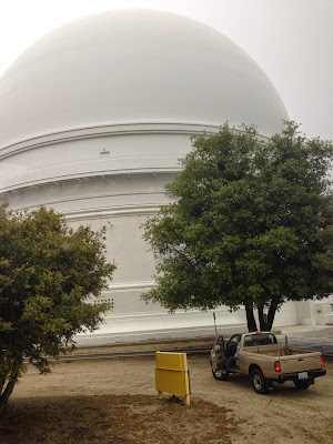
Today, I visited the Palomar Observatory in the mountains north of San Diego. Palomar has an extensive history of astronomical discovery throughout the twentieth century, and continues to be in use today. The observatory is home to a massive 200 inch telescope built and operated by Caltech. The size of the telescope—200 inches—refers to the diameter of the primary mirror of the telescope, and is a good measure of a telescope’s light collecting power. A series of five other mirrors help to focus the light and direct it to various instruments, including a spectrometer, the housing of which I was allowed to climb inside! The entire assembly itself is housed in a massive dome with the same diameter of the ancient Roman Pantheon. Our tour guide stressed that the huge dome and extensive support structures were all designed to protect and align a thin layer of aluminum weighing only five grams in total.

Unlike the everyday mirrors in bathrooms which owe their reflectivity to silver surfaces, Palomar uses aluminum to create its mirrors. Silver mirrors use a simple chemical process to coat glass, called the Tollen's test. At Palomar, aluminum deposition onto its glass primary is carried out in a precisely controlled vacuum environment in order to ensure the mirror is devoid of imperfections. When making telescopes, minuscule imperfections can be a big problem. Any deviation from a perfectly parabolic surface will scatter or blur the valuable image the telescope aims to collect. Imperfections of sizes comparable to the wavelength of the observed light (in this case, visible light, which is several tenths of a micron in wavelength) can compromise the instrument. Much care is taken in order to hunt down these tiny flaws on a giant mirror for this reason. Every two to three years, the aluminum on the mirror is carefully stripped and recoated using the same high-precision process in order to repair the accumulation of dust and foreign material (read: bird droppings) that accumulate from nightly use. 

Below are some panoramas I took from various locations under the dome. The primary mirror is located under the big structure and is currently pointed straight up. The large cylindrical tank is the vacuum chamber where the mirror is repaired.

Here is a view from the south end of the telescope. The hole on the left is where I got to enter the telescope. The cage on the top of the telescope is the observing platform, and is separated from the rest of the telescope in order to isolate the vibrations of whoever was observing. Today, electronic instruments take data instead of astronomers' eyes. 

What Does Europa Taste Like?

Today, I attended a lecture by Mike Brown, a Caltech professor most famous for "killing Pluto" by discovering the Kuiper Belt object Eris. This time, he was talking about his current scientific project: learning about the chemistry (and taste!) of Europa. One of the great things about being a Caltech undergrad is that I get to attend talks like this from world-class scientists without travelling too far from home!

Europa is an icy moon of Jupiter that is about the size of our own moon. Often, we hear that Europa is exciting because it has a subsurface ocean. Brown's rationale for studying Europa is a bit more nuanced than that--Ganymede, another moon of Jupiter, also has a reserve of liquid water underneath its surface but is less interesting to Brown's research because it has more water than Europa. This is because Ganymede has a thick enough liquid water ocean that towards the bottom, the pressure is high enough for the water to freeze out into ice. If you could slice into Ganymede, you would discover an object with an icy outer shell, a liquid water ocean, an inner icy shell and a rocky core, or as Brown described it, "an icy water sandwich." In contrast, the smaller water ocean cannot produce ice at the bottom of the ocean. Water can come in contact with Europa's rocky core, creating a boundary or "interface" where water and rock can interact chemically.

A water-rock interface is important because here on Earth, the interaction of water and rock drives plate tectonics and creates hydrothermal vents inhabited by some of the planet's most exotic creatures.

Water and ice also interact with Europa's surface, producing linear features on its surface and jumbled terrains that resemble icebergs floating on a frozen ocean. These features are produced by upwelling of water from Europa's subsurface ocean. Brown is currently working on identifying the chemical composition of salts present in these features. By doing so, he can sneak a peek at the composition of the ocean beneath. Here on Earth, the main salt in our oceans is sodium chloride. Is this true of Europa, too?

Using spectroscopic measurements from the massive Keck Telescope on the Big Island of Hawai'i, Brown can find out. Europa has a quite varied landscape, with three main compositions roughly corresponding two hemispheres and their border. Europa is tidally locked to Jupiter like our moon is, so one side always faces the giant planet. On the side that leads the planet on its orbit, only pure water ice is detected. On the trailing side, Brown found traces of sulfuric acid, produced by the interaction of sulfur ions from another Jovian moon, Io, carried to Europa by Jupiter's massive magnetic field. Between these two extremes, the surface water is laced with magnesium, potassium, and sodium salts that likely originate from the interaction of the water ocean and rocky core of Europa.

What does this mean for the taste of Europa? Brown suggests a mixture of ice, salt, and grapefruit juice--the sour citric acid in grapefruit replacing the harsher sulfuric acid--for a drink that is out of this world.